SplatBench

SplatBench is a direct test of spatial reasoning. A language model rebuilds an object from a few photos by placing every 3D Gaussian by hand, with no code or optimizer, and we grade the result from camera angles it never saw, so only a correct 3D structure scores well.

SplatBench is on Hugging Face: browse it in SplatBench Explorer, or load it from the SplatBench dataset.

A gradient-descent fit does the same job in a couple of minutes, so making 3D content this way is absurd, rather like painting a portrait by reading out brushstroke coordinates over the phone. As a measurement it is clean, because nothing else in the loop can do the reconstruction: every coordinate, size and angle in the scene comes from the model reading the photos and reasoning about space.

GPT-6 Astra is the strongest model we tested by a clear margin, followed by GPT-6.1 Sol and Claude Opus 5.5. Most other models score about as well as a single Gaussian painted in the object's average color, and even Astra falls short of a gradient-descent fit that uses a fifth of its Gaussian budget.

More reasoning effort raises almost every model's score, and its price varies widely between models. GPT-6.1 Sol at maximum effort beats GPT-6 Astra at medium effort for less than half the cost, and only Astra at its own maximum effort scores higher.

Why rebuild a splat by hand: it tests spatial reasoning without an optimizer

Language models pick up a surprising amount of spatial knowledge from text and images. One probe, "How 12 blind Claudes see the Earth", asks successive Claude models "land or water?" for a grid of latitude and longitude pairs given as plain text and plots each answer as a pixel: the older models draw noise, and Claude Opus 5.5 draws a clean world map. GeoGuessr environments test the opposite direction, from a street photo to a pin on the map.

SplatBench applies the same idea to objects. The input is a set of photos and the output is a 3D model built from primitives, where each primitive has a position, three scales, a rotation, a color and an opacity. For a good score, these values must agree with each other in 3D and with every photo at once, so the task measures how precisely a model can turn what it sees into coordinates, and how well it plans and corrects a long sequence of edits through tools.

LEGO-based benchmarks are the closest relatives, since they also ask a model to assemble an object from parts. Bricks come in a few sizes, fit together in a few orientations and snap onto each other through their studs, which gives a model structure to lean on. For Gaussians, position, size and angle vary continuously within the scene bounds, neighboring Gaussians blend into each other, and nothing in the parts corrects one that is misplaced.

3D Gaussian splatting represents an object as overlapping colored ellipsoids

Splatting is the graphics term for drawing a 3D point by spreading its footprint onto the image, like a splat of paint. 3D Gaussian splatting (Kerbl et al., 2023) represents a scene as a set of 3D Gaussians. Each Gaussian has a center $\boldsymbol{\mu}$, a covariance $\Sigma$ that sets its size and orientation, a color $c$ and an opacity $o$. Its density at a point $\mathbf{x}$ is

where $S = \operatorname{diag}(s_x, s_y, s_z)$ holds the three scales, which are standard deviations along the Gaussian's own axes, and $R$ is its rotation. These are the numbers a model writes in SplatBench.

To render a view, each Gaussian is projected to a 2D Gaussian on the image with covariance $\Sigma' = J W \Sigma W^{\top} J^{\top}$, where $W$ is the camera rotation and $J$ is the Jacobian of the perspective projection. The renderer sorts the projected Gaussians by depth and alpha-composites them front to back, so a pixel's color is

where $\alpha_i$ is the opacity of Gaussian $i$ times its projected 2D density at that pixel, and the white background fills whatever transmittance is left. Real captures use millions of Gaussians with view-dependent color. SplatBench allows up to 300, each with one flat color, which is enough for a recognizable object and few enough that a model can keep track of every Gaussian it has placed.

Balls fill volumes, discs make surfaces such as a tabletop, and needles make legs, rods and edges. A needle tilted along one camera's line of sight can look right from that camera and still draw a long streak across every other view.

The environment: the model edits a scene through tools, and a hidden grader scores it

An episode is a loop between the model and the environment. The model starts with the reference photos and the budgets and then calls one tool at a time; each call returns text, and the render tools also return an image. The environment checks every call, applies it to the scene and counts it against the budget. When the model submits or runs out of calls, a grader that the model never sees renders the scene from held-out cameras and computes the score, and a trajectory log keeps every call, the scene after every edit and the hidden score at that step.

Build task: the model writes every Gaussian through tool calls

Each episode starts with reference photos of one object, taken from cameras spread around it. Every photo shows the scene bounds, a cube from −1 to 1 on each axis, as a grey wireframe with an axis marker in the corner, so the model always knows which way is up and where each camera stands.

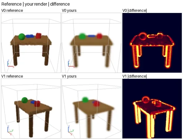
The model acts only through tools. It can add, edit and delete Gaussians, move or rotate a labeled group as one rigid piece, list its Gaussians and look at the photos again. To check its work, it renders its scene from reference cameras and gets each render back next to the photo, with a difference image and the PSNR, SSIM and silhouette IoU for that view. It can also render its scene from any other angle, though the tool returns no photo to compare with there. The environment specification lists every tool with its arguments and costs.

The budgets are tight on purpose: 300 Gaussians, 40 tool calls and 16 renders per episode. Here is the start of GPT-6 Astra's first build call on the table, shortened:

add_gaussians({ "gaussians": [
  { "pos": [-0.69, -0.51, -0.46], "scale": [0.065, 0.066, 0.31],
    "color": "#614019", "group": "legs" },
  // … 7 more legs
  { "pos": [-0.68, -0.48, 0.10], "scale": [0.11, 0.11, 0.037],
    "color": "#805e31", "group": "top" },
  // … 62 more pieces of tabletop
  { "pos": [-0.40, -0.12, 0.30], "scale": 0.127,
    "color": "#15952d", "group": "ball" },
  { "pos": [0.36, 0.03, 0.26], "scale": [0.096, 0.096, 0.102],
    "color": "#b51c20", "group": "red" },
  { "pos": [0.00, 0.23, 0.175], "scale": [0.16, 0.10, 0.055],
    "color": "#1c3aba", "group": "blue" }
]})

In this first call, working only from the photos, Astra puts the green ball within about two pixels of its true position in the photos. Its legs are right from side to side but too far apart from front to back, an error it finds and fixes later in the episode.

Reassembly task: the model moves the scrambled parts of a fitted splat back into place

The second task starts from a finished splat. We fit 300 Gaussians to the reference photos with gradient descent, cluster their centers into six parts with k-means, then move each part to a random place and rotate it about the vertical axis by 45° to 180°. The part labels are shuffled, so a label says nothing about where its part belongs, and the model has to find each part's position and heading from the photos and move it back with transform_group. Because the shapes are already right, this task measures placement and rotation on their own. A scrambled start scores far below zero.

Scoring: image metrics on held-out views, normalized against gradient descent

When the model submits, we render its scene from held-out cameras and compare each render with the real photo from the same camera, using PSNR for pixel error, SSIM for local structure and LPIPS for perceptual distance. For the procedural objects, the held-out cameras sit at angles where no reference photo was taken, some near the ground and some looking down.

Grading on held-out views closes the obvious shortcut. On the reference views alone, a model could score well by painting a flat picture in front of each camera, and such a picture looks wrong from every other angle.

The gradient-descent reference runs 2,000 Adam steps on an L1, SSIM and silhouette loss over the reference views, initialized on the visual hull (the volume consistent with every reference silhouette). Raw image metrics are also hard to compare across objects: an empty white scene already scores well on a small object, and some objects are much harder to fit than others. We therefore place each metric between two fixed points, an empty scene and a gradient-descent fit with the same 300-Gaussian cap and the same reference photos as the model. The fit gets 2,000 optimizer steps where the model gets 40 tool calls.

Each metric is averaged over the held-out views, and for LPIPS, where lower is better, the numerator and denominator are both negative, so the same formula holds. A score of 0 matches an empty scene and 100 matches the optimizer. Scores below zero are common because misplaced Gaussians cover white background that an empty scene gets right, and since the fit is not optimal, scores above 100 are possible.

Task set: procedural shapes, NeRF-Synthetic models and photographed real objects

The procedural objects are built from spheres, boxes, cylinders and cones, so their 3D ground truth is exact: a snowman, a mushroom, a table, a rocket, a tree and a robot. The synthetic objects come from the NeRF-Synthetic dataset: the LEGO bulldozer, the chair, the hot dog, the ficus, the microphone and the drum kit. The real objects are photographed captures: the Ignatius statue and the Caterpillar excavator from Tanks and Temples, and a jade carving from BlendedMVS. Every object appears both as a build task and as a reassembly task.

Results: most models score near a single Gaussian, and the best still trail a small optimizer fit

Each model ran every task twice at medium reasoning effort. GPT-6 Astra beats GPT-6.1 Sol on almost every task, and Sol beats Claude Opus 5.5 on almost every task. Below them the scores drop sharply, and the remaining models all score near a single Gaussian in the object's average color, with most of the differences among them within noise.

Model	SplatScore [95% CI]	Cost per episode	Time per episode
GPT-6 Astra	49.6 [41.4, 58.0]	$1.69	6.5 min
GPT-6.1 Sol	38.6 [30.6, 46.3]	$0.27	5.1 min
Claude Opus 5.5	25.0 [17.1, 32.6]	$0.71	5.0 min
GPT-6 Luna	8.6 [1.8, 15.2]	$0.02	4.5 min
Claude Sonnet 5.5	5.7 [0.2, 10.6]	$0.04	0.7 min
Claude Haiku 5.5	3.6 [−5.8, 12.4]	$0.01	1.9 min
Grok 4.7	2.1 [−8.8, 11.8]	$1.38	24.0 min
GPT-5.6 Terra	1.2 [−7.4, 9.4]	$0.19	2.1 min

GPT-6.1 Sol reaches about four fifths of Astra's score at about a sixth of its cost. Grok 4.7 is the second most expensive model and by far the slowest, and it scores at the level of a single Gaussian.

Detailed objects are much harder than procedural shapes

On the procedural shapes, Astra comes close to gradient descent with 64 Gaussians, and Astra and Sol beat it on a few procedural tasks. On the NeRF-Synthetic and real objects, every model falls far below that fit, and the Caterpillar excavator is the hardest object overall. These objects have fine detail and texture that a few hundred flat-colored Gaussians written by hand cannot reproduce, and since the renderer has no lighting, the model also has to paint the shading into its colors.

Reassembly: the strongest models turn the parts back to their true heading

Reassembly takes shape out of the problem: the parts are already correct, and the model only has to move and turn them. Astra and Sol score higher on reassembly than on building, and Opus and Luna score lower. Comparing each part's final pose with its true pose shows the difference. Astra turns more than half of the parts back to within 15° of their true heading and Sol about a third, while Opus and the other models turn few parts back.

Weaker models build blobs that fit the object's mirror image as well as the object

A rough blob in the right place can score above zero without capturing any of the object's shape. To test for shape, we mirror each finished build across a vertical plane and measure its overlap with the held-out silhouettes again. The builds of Astra, Sol and Opus lose a clear share of their overlap, so they follow the object's actual layout. The other models lose almost none, which means their builds fit the mirrored object about as well as the real one, and several of them also build the object too small.

The strongest models improve until the end of the episode, and Grok makes its scenes worse

Astra, Sol and Opus are still gaining in the second half of the episode. The first builds of Terra and Haiku score below an empty scene, and they spend the episode recovering. Grok's scenes peak around halfway and then degrade: it usually runs out of tool calls while it is still editing, and on average it submits a scene 20 points below the best one it had.

Reasoning effort: higher effort raises scores, and the cost grows faster than the gain

The leaderboard runs every model at medium reasoning effort. To see how much of the gap between models comes from that setting, we ran all of them except Grok 4.7 again at high and at maximum effort on half of the tasks, which is why the medium scores below differ slightly from the leaderboard.

Model	Medium	High	Max	Cost per episode at medium	Cost per episode at max
GPT-6 Astra	51.8	55.8	61.6	$1.90	$5.15
GPT-6.1 Sol	43.9	47.6	56.8	$0.30	$0.90
Claude Opus 5.5	31.5	33.1	45.4	$0.75	$6.53
Claude Sonnet 5.5	7.4	18.7	35.3	$0.02	$5.00
Claude Haiku 5.5	9.2	6.2	20.9	$0.01	$0.21
GPT-6 Luna	17.5	14.8	20.8	$0.02	$0.05
GPT-5.6 Terra	4.3	10.8	18.2	$0.20	$0.96

At maximum effort almost every model scores higher and the order at the top does not change, but the cost per episode rises much faster than the score, up to 250-fold for Sonnet, and the longest episodes run for most of an hour. GPT-6.1 Sol at maximum effort beats GPT-6 Astra at medium effort for less than half the cost, and only Astra at maximum effort scores higher than it. Claude Opus 5.5 at maximum effort scores about the same as Sol at medium effort, at about twenty times the cost.

Claude Sonnet 5.5 stops early at medium effort, and higher effort keeps it working

At medium effort Sonnet usually places a handful of Gaussians in a single call and submits without looking at a render. Its own summary of one such episode reads: "I never rendered it or compared it against the reference photos, so its accuracy is unchecked." Asking it to continue does not help. When we refused its first early submit and reminded it that the score comes from views it has not seen, it submitted again at once with the same score, and the same was true of the other models that stop early. At higher effort it keeps working on its own, and its score rises from 7 at medium to 35 at maximum, from near the bottom of the table to fourth.

Higher effort also changes how the Claude models work. At maximum effort they often begin by placing a few temporary Gaussians, rendering them to see where they land in the photos and deleting them before they build, a check they never make at medium effort.

One-shot reconstruction: the leading models are level on a first attempt, and feedback separates them

In one-shot reconstruction, the model sees the photos and gets a single tool call: it has to place every Gaussian at once, with no chance to render the scene or correct it.

Every model does worse in one shot, Astra by 40 points and Sol by almost 30. On the one-shot attempt, GPT-6 Astra, GPT-6.1 Sol and Claude Opus 5.5 are statistically level, so Astra's lead in the full episode comes from how it uses render feedback.

Trajectories: how the models build and reassemble scenes, call by call

Every episode can be replayed call by call, with the hidden held-out score after each edit. In the replays below, Astra blocks out the table's structure first and then corrects it from render feedback, and Luna keeps adding detail on top of an armchair whose base never works. Sonnet builds the same mushroom once in a single call and once in a long render-and-edit loop, and in the robot reassembly the strongest models differ in how they handle rotation.

GPT-6 Astra builds the table's frame first, then fixes it from render feedback

Astra's first build call lays out the whole table: tall Gaussians for the legs, a grid of flat ones for the tabletop and a placeholder for each object on top. One render later it deletes the legs and the placeholders and rebuilds them from smaller pieces, then raises the tabletop slightly, adds an edge band and lifts the book onto the surface.

After comparing its renders with the photos, Astra pulls the front and back edges of the tabletop inward and moves the front and back legs toward the middle in the two marked calls. With the legs standing where the real legs do, the held-out score jumps from 41 to 68, the largest gain of the episode. Most of its later calls adjust the ball, the cup and the book or add detail such as lower leg segments, a rim and wood grain. Like a carpenter, it settles the frame before it works on what stands on it.

GPT-6 Luna starts with oversized Gaussians and never repairs that base

In its first two calls on the armchair, Luna lays down the seat, the back, the arms and the legs as large flat slabs and long needles. It appears to set each scale to the half-width of the part it wants, but a scale is a standard deviation, and a Gaussian keeps rendering well past one standard deviation, so these first Gaussians come out far too large. The seat alone spreads wider than the whole chair, and the tails streak across the held-out views and push the score below zero.

Luna never repairs this base. It edits the first Gaussians several times, mostly to make them thinner, but a thinner needle reaches almost as far. Meanwhile it adds a couple of hundred smaller Gaussians of detail on top, such as a seat pattern, carvings, fabric and an apron, and it renders after almost every change until its render budget is gone, while its score stays near zero.

Claude Sonnet 5.5 guesses the mushroom at medium effort and builds it carefully at maximum effort

At medium effort, Sonnet places 11 Gaussians for the stem, the cap and its spots in one call, and submits at 6.7 without rendering. The whole episode takes 10 seconds and costs about a cent.

At maximum effort, on the same task, it first places a group of temporary Gaussians that it names calib, renders them and deletes them. It then builds the cap and the stem, renders, and rebuilds the whole mushroom. Most of its remaining calls go to the spots: it adds a batch, renders and deletes it again several times before it keeps one, and it ends with small edits to the cap. The call budget ends the episode at 78.4, after 54 minutes and $5.98.

Robot reassembly: Astra restores the body and leaves one symmetric leg backwards

The scrambled robot starts at −62. In its first run, Astra inspects the parts before moving anything: it asks for a summary of the groups, renders the parts from two cameras and lists their Gaussians. It then moves and rotates each part into place with a single transform_group call, taking the score from −62 to 65 within six calls, and small corrections bring it to 92.

The table gives each part's final heading error in the first run, with left and right as seen from the front.

Part	GPT-6 Astra	GPT-6.1 Sol	Claude Opus 5.5	GPT-6 Luna
Head	0°	0°	0°	2°
Left arm and torso	3°	2°	3°	57°
Right arm and chest	5°	3°	11°	45°
Right lower torso	0°	3°	3°	32°
Left leg	4°	94°	61°	61°
Right leg	179°	106°	118°	118°
Final score	92.1	72.3	61.1	33.8

Astra rotates five of the six parts to within 5°. The sixth, the right leg, ends up facing backwards: the legs are plain boxes that look almost the same after a half turn, so both headings fit the photos about equally well. In this run Astra also swaps the two legs, which costs little because they look alike. Near the end it tests the other heading by turning both legs half a turn and rendering, sees the renders get worse and turns them back.

Sol turns the four body parts to within 3°, and it rotates the legs as well, but both end up about 100° from their true heading. Opus gets the head and the body parts to within about 10°, but it swaps two of the body parts and moves the legs without rotating them. Luna first rotates two parts by exactly half a turn. Its later corrections bring the head close to its true heading, but the other three body parts end up misplaced and 30° to 60° off, and it never rotates the legs.

Every episode can be replayed

Every episode can be replayed in the same player, at each effort level, with the early submit refused and in one shot. The dots in Figure 1 and the scores in the results table open their episodes here.

Environment specification: interface, tools, limits and reward

The benchmark is a fixed task set run through an environment built for reinforcement learning. Each tool call is one step that returns text and sometimes an image, and the reward arrives once, at the end of the episode.

Interface: reset, one tool call per step, terminal reward

env = SplatEnv(device="cuda")
obs = env.reset(task)               # obs.text: cameras and budgets; obs.image: reference sheet
out = env.add_gaussians([...])      # every tool returns ToolOut(text, image=None, done=False)
out = env.render_views(views=[0, 1, 6, 7])
out = env.submit()                  # out.done is True
reward = env.get_reward()           # benchmark reward: clip(SplatScore / 100, 0, 1)

A task is a small spec. For reassembly, init_npz points to the scrambled Gaussians and their group labels. One-shot reconstruction sets max_tool_calls to 1 and max_renders to 0.

{ "task_id": "table__sculpt", "kind": "sculpt",
  "max_gaussians": 300, "max_tool_calls": 40, "max_renders": 16, "init_npz": null }

Observations, actions and budgets

Field	Specification
Observation	Text after every call. view_references, render_views and render_angle also return one PNG.
Action	One tool call with JSON arguments, validated against the tool's schema.
Gaussian	pos in [−1.25, 1.25]³; scale in [0.005, 0.5]³ as standard deviations, or one number for a sphere; rotation as XYZ Euler degrees or a quaternion; color as #rrggbb or RGB; opacity in [0.05, 1]; an optional group label.
Start	Build: an empty scene. Reassembly: 300 Gaussians in six labeled groups, each moved and rotated about Z.
Images	Scenes are 256 × 256 pixels on white. The model gets them as labeled contact sheets with the bounds cube and an axis marker drawn on.
Budget	300 Gaussians, 40 tool calls and 16 renders; one call and no renders in one-shot reconstruction.
End	submit, or an automatic submit when the call budget runs out.
Reward	Terminal, from the held-out SplatScore: clip(score / 100, 0, 1) for the benchmark, and a shifted mapping for training (see below).

The first observation is the reference sheet and this text:

Reference views: V0 (azimuth 0°, elevation 20°), V1 (azimuth 60°, elevation 20°), …,
V7 (azimuth 210°, elevation 65°). The image shows all reference views. Budget: at most
300 Gaussians, 40 tool calls, 16 renders. The scene starts empty. Build the object from Gaussians.

Tools for editing, inspecting, rendering and submitting

Tool	Arguments	Returns	Cost
add_gaussians	list of {pos, color, scale?, rot?, opacity?, group?}	the new ids	1 call
edit_gaussians	list of {id, …fields}	the number edited	1 call
delete_gaussians	ids or group	the number deleted	1 call
transform_group	group or ids; translate, rotate_deg, scale about the set's centroid	old and new centroid	1 call
list_gaussians	optional group	one text row per Gaussian	1 call
describe_groups	none	count, centroid, bounding box and mean color per group	1 call
view_references	optional views	the reference sheet	1 call
render_views	optional views, groups	photo, render and difference per view; PSNR, SSIM, silhouette IoU	1 call, 1 render
render_angle	azimuth, elevation, optional groups	a render from any orbit angle, with no photo	1 call, 1 render
submit	none	ends the episode	1 call

Every result ends with the remaining budget, so the model always knows where it stands:

render_views(views=[0, 1, 6, 7])
Metrics on reference views: V0: PSNR 18.62 dB, SSIM 0.843, silhouette IoU 0.800;
V1: PSNR 14.49 dB, SSIM 0.792, silhouette IoU 0.597; V6: …; V7: …
[74/300 Gaussians | calls left 37 | renders left 15]

Validation: an invalid call changes nothing and still costs a call

Calls are atomic: if any Gaussian in a call is invalid, nothing changes and the call returns the reason, and it still uses one of the 40 calls. Positions outside the bounds and calls that would exceed the Gaussian budget are rejected, scales are clamped with a warning, and opacity is raised to its floor. In this real example from GPT-6 Astra on the snowman, one mistyped color voided a whole batch:

ERROR: nothing was added. #28: unknown color '#cacc cb' (use '#rrggbb' or [r,g,b])
[17/300 Gaussians | calls left 36 | renders left 15]

Held-out views, scores and the reference fit never reach the model

The metrics in render_views come from the reference views, which the model already has. The held-out views, the held-out score and the gradient-descent fit never pass through any tool, because a visible held-out score would let a model raise it by trial and error against the grader, and the benchmark would then measure search. The part labels in reassembly are shuffled for the same reason, so a label carries no hint of position.

Trajectory logs: every call, plus scene snapshots and hidden scores

Every call is logged with its arguments and the text it returned. After every call that changes the scene, the log also stores a full copy of the scene and the held-out metrics, which the model never sees. These records drive the replays in this post. The environment's reward stays terminal; the per-step metrics are logged for analysis and can be used as process rewards or for credit assignment in your own training setup. An example record, shortened:

{
  "step": 17,
  "tool": "transform_group",
  "args": { "ids": [92, 93, …, 109], "translate": [0, -0.11, 0] },
  "text": "Transformed 18 Gaussians about their centroid [-0.0, 0.51, -0.44]; new centroid [-0.0, 0.4, -0.44]. [208/300 Gaussians | calls left 23 | renders left 13]",
  "hidden": { "score": 68.14, "psnr": 22.50, "ssim": 0.902, "iou": 0.929, "lpips": 0.213 },
  "state": [ { "id": 8, "p": [-0.68, -0.408, 0.155], "s": [0.075, 0.075, 0.025],
               "q": [1, 0, 0, 0], "c": [0.502, 0.369, 0.192], "o": 1.0, "g": "top" }, … ]
}

Renderer: a differentiable EWA rasterizer in plain PyTorch

The renderer is a dense EWA (elliptical weighted average) splatting rasterizer in plain PyTorch. It projects each Gaussian with the clamped Jacobian used in 3D Gaussian splatting, adds a 0.3 px² low-pass dilation, sorts by depth and composites front to back, with α clamped to 0.99 and discarded below 1/255. Because it is differentiable, the same code fits the gradient-descent reference and grades the models, and it needs no custom CUDA kernels.

Training with TRL: one environment per GRPO rollout and a shifted reward

SplatTRLEnv adapts the environment to TRL's environment_factory, so each GRPO rollout gets its own environment and calls the same tools. Dataset rows carry a task_path, and complex arguments travel as JSON strings, which small open models tend to produce more reliably than nested argument schemas.

trainer = GRPOTrainer(
    model=model,
    train_dataset=Dataset.from_list([
        {"prompt": [{"role": "user", "content": "Rebuild the object."}],
         "task_path": "tasks/snowman__sculpt.json"},
        # …
    ]),
    environment_factory=SplatTRLEnv,
    args=GRPOConfig(max_tool_calling_iterations=24),
)

For training, the reward is shifted so that scenes worse than empty still rank against each other: $r = \operatorname{clip}\big((\text{SplatScore} + 50)/150,\ 0,\ 1\big)$, where an empty scene earns one third and the gradient-descent fit earns 1. With the benchmark's clipping at 0, a GRPO group of weak rollouts would often score 0 throughout and produce no advantage signal.

SplatBench as an RL environment: a verifiable reward over long, feedback-driven episodes

The score is continuous and verifiable: every scene gets a graded score from image metrics against held-out photos, with no rubric and no model acting as judge, so partial progress earns partial credit. Episodes are long multi-turn loops in which the model renders, compares its render with the photos and edits, and one-shot reconstruction shows that most of the score comes from this loop. The task is far from saturated: even the best model at maximum effort stays below gradient descent with 64 Gaussians, and most models score near a single Gaussian. New tasks are cheap to make, since the procedural objects and a generator of random multi-object scenes come from code, so training tasks need no manual authoring and the benchmark objects can stay held out.

The per-step hidden scores make the trajectories useful beyond their final score. They show where an episode went wrong, which a terminal reward cannot: Grok's builds end well below their best intermediate scene, and the step where each one turned is in the log. The effort sweep adds paired trajectories of the same model on the same task at different reasoning budgets, such as Sonnet's two mushrooms above.

Design decisions: what each choice rules out

Most of these choices stop a model from scoring well without doing the spatial reasoning the benchmark is meant to measure.

• No code interpreter. With code execution, a model would write a small optimizer, and the test would measure coding.
• Hidden, held-out grading. Flat pictures painted for the reference cameras do not transfer to other angles, and the grade never reaches the model (see the environment specification).
• A matched optimizer as the 100 mark. Normalizing by a fit with the same Gaussian cap and the same photos puts objects of very different difficulty on one scale.
• Small budgets. Three hundred Gaussians are enough for a recognizable object and few enough to keep track of, and forty calls with sixteen renders leave room for several rounds of feedback while keeping an episode of the leading models at medium effort to a few minutes.
• Bounded objects on a turntable. A bounded object has a clear inside and outside, cameras that circle it and a ground truth we can check. Open scenes would add problems of scale and occlusion that we want to study separately.
• Flat colors and a drawn frame. Flat colors keep each Gaussian to a few plain numbers, as in the simplest form of splatting, and the bounds cube, the axis marker and the stated conventions remove guesswork about orientation.

Limits and evaluations in progress

Two runs per task make comparisons on a single task noisy, so every comparison in this post uses the whole task set, and the set of real objects is too small to read as a separate ranking. The objects are bounded and centered, colors are flat and images are small, so the benchmark says little about lighting, materials or open scenes. There is no human baseline yet.

We are now working on larger Gaussian and call budgets, more runs per task and scenes with several objects, and we will add the results to this page as they finish.

Access to the environment, tasks and trajectories, and citation

The environment, the task set and the trajectories of all 1,230 episodes, including every intermediate scene and its hidden score, are available to teams that train or evaluate models on spatial and visual tasks. To get access, write to founders@vibemotion.ai.

@misc{perpetual2026splatbench,
  title  = {SplatBench: Raw Spatial Reasoning by Placing 3D Gaussians},
  author = {{Perpetual Research}},
  year   = {2026},
  url    = {https://perpetualresearch.si/splatbench}
}